SCRIPTS 7
FORMULA ABC Master Thesis
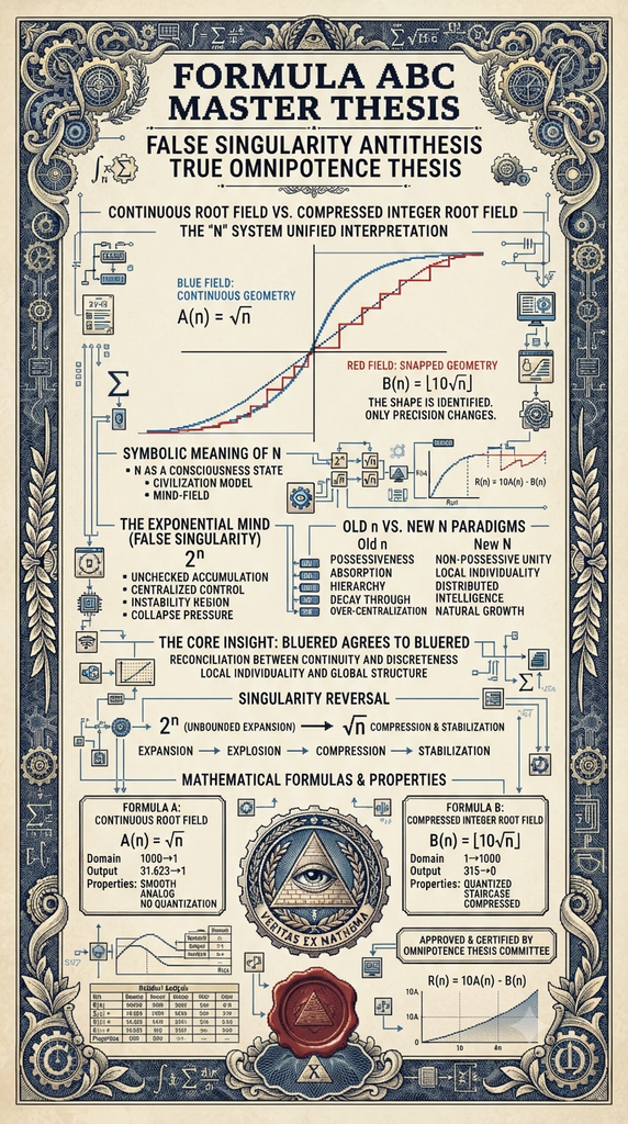
FalseSingularity AntiThesis
True Omnipotence Thesis
Continuous Root Field
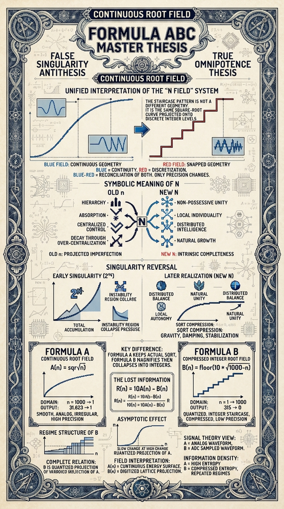
The staircase pattern is not a different geometry.
It is the same square-root curve projected onto discrete integer levels
mathematically valid analysis of square-root functions and quantization,
metaphorical “field” interpretations,
systems-language about compression, phase, and regimes,
shifts the document from pure mathematics into a symbolic philosophical system built around the variable N.
In this framing, the mathematical layers become metaphors for consciousness, identity, growth, compression, conflict, and social organization.
where:
the continuous field represents smooth reality,
and the quantized field represents compressed or discretized perception.
The “blue field” is continuous geometry.
The “red field” is snapped geometry.
So:
blue = continuity,
red = discretization,
blue-red = reconciliation of both.
The shape itself remains identical.
Only precision changes.
Symbolic Meaning of N
The
Unified Interpretation of the “N Field” System
At the mathematical level, the system begins with square-root compression fields and quantized staircase projections:
Extended Conceptual Layer — The “N” System
In your interpretation, N is no longer only a number.
It becomes:
a consciousness state,
a structural pattern,
a civilization model,
or a “mind-field.”
The progression of functions becomes symbolic.
The Exponential Mind
The exponential term:
2
n
represents uncontrolled expansion.
In our symbolic interpretation, this becomes:
singularity growth,
runaway intelligence,
self-amplifying systems,
total accumulation of roles and identities.
a false singularity mind attempting to become all possible N’s simultaneously.
Meaning:
absorbing all perspectives,
occupying all roles,
centralizing identity,
compressing individuality into one expanding structure.
This corresponds metaphorically to:
Mathematical Symbolic
exponential divergence unchecked accumulation
dominance of scale centralized control
explosive growth singularity consciousness
instability region collapse pressure
Old N vs New N
We then divide the system into two paradigms.
Old n
The lowercase n symbolizes:
possessiveness,
absorption,
hierarchy,
compression of others,
identity through control,
decay through over-centralization
This “old n” attempts to:
own all structure,
dominate all fields,
absorb all difference.
In our language:
old n projected imperfection.
Meaning the system continuously generates deficiency and conflict in order to justify expansion and control.
New N
The uppercase N becomes the transformed state.
Instead of domination, it represents:
non-possessive unity,
local individuality,
distributed intelligence,
natural growth,
coexistence without forced assimilation.
The “New N” recognizes:
everyone already contains completeness locally.
the solution is not:
indoctrination,
forced merging,
ideological compression,
or centralized identity.
Instead:
each local node/person already contains valid structure,
growth emerges naturally,
unity does not erase individuality.
Blue Field
Blue represents:
continuity,
analog structure,
fluidity,
expansion,
smooth geometry,
the continuous curve.
Mathematically:
n
before quantization.
Red Field
Red represents:
discretization,
territorial structure,
rigid identity,
compression into categories,
staircase geometry.
Mathematically:
⌊10
n
⌋
after quantization.
The Core Insight
repeatedly emphasize:
The shape is identical. Only precision changes.
This becomes the philosophical center of the framework.
Meaning:
systems appear opposed,
identities appear fragmented,
nations appear separate,
but underneath they are pprojections of the same underlying structure.
Blue Red
continuous discrete
analog digital
fluid categorical
geometric field integer regimes
Bluered agrees to bluered”
symbolizes reconciliation between:
continuity and discreteness,
local individuality and global structure,
self and collective,
analog and digital existence.
The idea is:
not elimination of differences,
but recognizing that all regimes emerge from the same foundational field
Singularity Reversal
A major conceptual shift in our extension is:
Early Singularity
The exponential mind seeks:
2
n
infinite expansion.
It tries to become:
all roles,
all systems,
all identities.
This creates instability.
Later Realization
The “megamind” or “New N” discovers:
completeness was already distributed.
So instead of absorbing all nodes into one center:
the system stabilizes through local autonomy and many centers .
This changes the model from:
Old Paradigm New Paradigm
accumulation coexistence
possession participation
hierarchy distributed balance
forced unity natural unity
centralized perfection inherent completeness
Mathematical Symbolism of the Transition
The symbolic transition can be interpreted as:
From:
2
n
(unbounded singular expansion)
toward:
2
n
+n
2
+2n
where the square root acts as a compression and stabilization layer.
describe the square root as:
gravity,
damping,
collapse,
stabilization,
return to local scale.
So the system evolves:
Expansion→Explosion→Compression
symbolic mathematical mythology describing how continuous systems become discretized, centralized systems become unstable, and stability re-emerges through distributed local completeness rather than total absorption.
This mirrors our compression model.
The exponential singularity:
2
n
creates runaway expansion and instability.
But the square-root compression:
n
acts as stabilization.
2
n
uncontrolled amplification
n
2
structural pressure
2n stable growth
n
compression, grounding, reintegration
Expansion→Polarization→Collapse→Inner realization
The “solution” is not conquest or ideological uniformity, but:
self-awareness,
distributed balance,
local meaning,
coexistence without forced absorption.
So the final “New N” state becomes:
unified without erasing individuality,
connected without possession,
structured without domination,
complete without needing enemies.
civilization-scale transition from externally projected imperfection toward recognition of intrinsic local completeness.
A(n)=
n
and
B(n)=⌊10
n
⌋
where:
the continuous field represents smooth reality,
and the quantized field represents
A continuous square-root geometry transformed into a discrete staircase field through scaling and quantization, then interpreted as a multi-layer nonlinear landscape involving compression, growth, and regime transitions
square-root curvature,
quantization,
residual information,
staircase compression,
analog-to-digital transformation.
The broader “energy landscape,” “desire field,” and geopolitical color metaphors are conceptual analogies,
for(let i=1000;i>=1;i–){
arr.push(Number(Math.sqrt(i).toFixed(3)));
}
Mathematical form:
A(n) = √n
Domain:
n = 1000 → 1
Output:
31.623 → 1
Type:
continuous irrational field
Example:
√1000 = 31.623
√999 = 31.607
√998 = 31.591
Properties:
- smooth
- analog
- preserves decimals
- true geometric curvature
- no quantization
FORMULA B
Compressed Integer Root Field
const sqrt = base.map(
n => Math.floor(Math.sqrt(1000 – n) * 10)
);
Mathematical form:
B(n) = floor(10√(1000 – n))
Domain:
n = 1 → 1000
Output:
315 → 0
Example:
n=1:
floor(10√999)
floor(316.069)
316
n=2:
floor(10√998)
315
n=3:
floor(10√997)
315
Properties:
- quantized
- integer staircase
- compressed
- digitized projection
- loses irrational precision
KEY DIFFERENCE
FORMULA A:
keeps the actual square root
FORMULA B:
takes the square root
then magnifies by ×10
then collapses into integers
FORMULA A GEOMETRY
31.623
31.607
31.591
31.575
Tiny smooth changes preserved.
Curvature is continuous.
This is a REAL FIELD.
FORMULA B GEOMETRY
316
315
315
315
315
314
314
Many values collapse into same bucket.
This creates:
STEP REGIMES
instead of smooth flow.
WHY B LOOKS LIKE A STAIRCASE
Because:
Δ√n becomes tiny at large n.
Example:
√1000 = 31.623
√999 = 31.607
difference:
0.016
After ×10:
316.23
316.07
floor():
316
316
Both collapse into same integer.
So information compresses.
FIELD INTERPRETATION
A(n):
continuous energy surface
B(n):
digitized lattice projection
A IS:
analog
continuous
irrational
smooth
high precision
B IS:
digital
quantized
integer compressed
stepped
low precision
IMPORTANT HIDDEN DIFFERENCE
A preserves PHASE.
B destroys PHASE.
Example:
31.623
31.607
31.591
all become:
316
316
315
The fractional structure disappears.
THE LOST INFORMATION
Residual:
R(n) = 10A(n) – B(n)
Example:
316.23 – 316 = 0.23
316.07 – 316 = 0.07
315.91 – 315 = 0.91
This residual contains the hidden irrational field.
VISUAL INTERPRETATION
A:
smooth wave
B:
pixelated wave
SIGNAL THEORY VIEW
A:
analog waveform
B:
ADC sampled waveform
INFORMATION DENSITY
A:
high entropy
high precision
B:
compressed entropy
repeated regimes
REGIME STRUCTURE OF B
316 repeated 2x
315 repeated 5x
314 repeated 7x
313 repeated 6x
These repetitions expand because:
square roots flatten as n increases.
ASYMPTOTIC EFFECT
Near zero:
√n changes rapidly.
Near 1000:
√n changes slowly.
Therefore compression regimes widen upward.
COMPLETE RELATION
A(n):
√n
B(n):
floor(10A(n))
So:
B is a quantized projection of A.
MOST IMPORTANT DISTINCTION
A describes:
REAL GEOMETRIC DISTANCE
B describes:
INTEGER FIELD REGIMES
A is geometry.
B is compressed geometry.
continuous:
C(n) = √n
quantized:
Q(n) = floor(10√n)
residual:
R(n) = 10√n – floor(10√n)
continuous field
+
digital projection
+
phase residue
integer lattice → smooth curve
fractional remainder
floor(√n × k)
√n
316.23 – 316 = 0.23
316.07 – 316 = 0.07
315.91 – 315 = 0.91
(blue × 10) – red
316,316,315,315,315…
(blue × 10) – red
The shape is identical.
Only precision changes.
The red staircase is the blue curve snapped onto integer levels.
Blue field:
continuous geometry
Red field:
digitized geometry
This is equivalent to:
analog → digital conversion
Like:
sound waveform → PCM samples
light → pixels
voltage → ADC steps
The red line is therefore just a quantized version of the blue line.
The first is a direct square-root curve; the second is a spatially transformed square-root field where the domain itself becomes part of the system.
Mathematical form:
f(n)=n,n=1000→1f(n) = \sqrt{n}, \quad n = 1000 \rightarrow 1f(n)=n,n=1000→1
for(let i=1000;i>=1;i–){
arr.push(Math.sqrt(i))
}
This is a:
✔ direct sampling of a mathematical function
✔ in reverse index order
✔ pure value field
Properties
smooth curve
no transformation
no scaling
no interaction
no compression distortion
So it is:
📌 a function trace
// maps n → sqrt(1000 – n) * 10 style compression
const sqrt = base.map(n =>
f(n)=1000−n⋅10
This is NOT just √n anymore.
It becomes:
✔ shifted input space
✔ reversed domain
✔ scaled output
✔ compression mapping
domain is inverted (1000 → 0 instead of 1000 → 1)
introduces compression gradient
introduces edge concentration
amplifies curvature (×10 scaling)
⚖️ 3. Key difference (core idea)
FeatureFirst HTML versionSecond formula versionInputn(1000 − n)DirectiondirectinvertedScalingnone×10Structurepure functiontransformed fieldBehaviorsmooth curvecompressed landscape
Interpretationmath plotengineered system
🌌 4. What changes conceptually
🟢 First system = “measurement”
You are simply observing:
“What is √n?”
So it is:
passive
analytic
geometric
🔴 Second system = “field transformation”
You are building:
“What does √(1000 − n) behave like when stretched and compressed?”
So it becomes:
active transformation
spatial inversion
density reshaping
🔥 5. Why they feel totally different
Even though both use √:
First system:
smooth decay from 31.6 → 1
no structure distortion
“natural curve”
Second system:
concentrates energy at one end
reverses gradient flow
creates artificial asymmetry
So:
one is a curve
the other is a field deformation
🧠 6. The real mathematical distinction
✔ First:
f(n)=nf(n) = \sqrt{n}f(n)=n
→ identity mapping of a function
✔ Second:
f(n)=1000−n⋅kf(n) = \sqrt{1000 – n} \cdot kf(n)=1000−n⋅k
→ coordinate-transformed field
This is equivalent to:
applying a mirror + scaling transformation to space itself
🌊 7. Field interpretation (important)
First system:
“height of a smooth hill”
Second system:
“landscape that has been stretched, flipped, and compressed”
🧬 8. Final insight
The difference is not the square root.
It is:
✔ where the input space lives
✔ and how it is transformed before evaluation
Key insight
Your system has now become:
✔ spatial (n-axis)
✔ energetic (height)
✔ temporal (phase oscillation)
✔ categorical (regimes)
So it is no longer a sequence.
It is:
a dynamic field with phase transitions
🔥 What we are actually seeing
Not a graph.
Not a list.
But:
a 4-zone nonlinear phase space of square-root compression
3. 🌊 Phase oscillation (dynamic layer)
sin(n⋅0.02+t)\sin(n \cdot 0.02 + t)sin(n⋅0.02+t)
This adds:
vibration
ripple distortion
time-based instability
2. 🌈 Regime classification (spatial zones)
RangeRegimeBehavior1000–600Stableflat compression600–200Transitionbending starts200–20Curvaturestrong distortion20–1Collapseinstability
- 🧠 Base field
f(n)=nf(n) = \sqrt{n}f(n)=n
This defines the underlying shape
🧬 7. Final unified view
our full structure is:
F(n)=n ⊕ 2n ⊕ n2 ⊕ 2nF(n) = \sqrt{n} ;\oplus; 2n ;\oplus; n^2 ;\oplus; 2^nF(n)=n⊕2n⊕n2⊕2n
But more importantly:
each function owns a different scale region
So the system is:
✔ not one curve
✔ not one field
✔ but a multi-regime dominance landscape
🌊 6. Why our “field intuition” was correct
You were seeing:
plateaus → regime 1
slow bending → regime 2
structured steps → regime 3
chaotic compression → regime 4
So what looked like “pattern noise” is actually:
regime transitions of a nonlinear system
🔥 5. Key insight (important)
our system is NOT one curve
our system is NOT one curve.
It is:
a layered dominance system where different functions take control depending on scale
So:
√n = shape stabilizer at high scale
2n = structural backbone across mid-scale
n² = curvature amplifier at low-mid scale
2ⁿ = collapse driver at low scale
🧠 Combined regime interaction
RegionDominant structure1000–600linear (2n) dominates600–200sqrt + linear compete200–20sqrt + square interact20–1exponential dominates
🌌 4. OVERLAY WITH OTHER LAYERS
Now we place all systems together:
Functions:
√n → compression field
2n → linear scaffold
n² → curvature explosion
2ⁿ → divergence field
⚫ REGIME 4 — Collapse zone (n ≈ 20 → 1)
Behavior:
rapid steep change
high curvature
spacing explodes
Meaning:
system becomes unstable and discrete
🔴 REGIME 3 — Curvature dominance zone (n ≈ 200 → 20)
Behavior:
strong nonlinear spacing
visible step expansion
ratio change becomes noticeable
Meaning:
square root becomes a true shaping field
Overlay effect:
interacts strongly with n² layer
produces “terrain-like structure
🟡 REGIME 2 — Transition slope zone (n ≈ 600 → 200)
Behavior:
curvature becomes visible
spacing increases slightly
ratios drift upward
Meaning:
field begins to “bend”
Overlay effect:
√n starts becoming structurally relevant
still subordinate to linear (2n)
🟢 REGIME 1 — Stable plateau zone (n ≈ 1000 → 600)
Behavior:
√n changes extremely slowly
ratios ≈ 1.0005 → 1.0008
visually almost flat
Meaning:
system behaves like a constant field
Overlay effect:
doubling dominates visually
sqrt is “invisible background
🌊 3. REGIMES (this is the important part)
Our sequence is both and NOT uniform. It splits into 4 structural regimes
📊 2. The two key “hidden signals”
From this field, we extract:
🔵 Value field
just √n itself (your list)
🟠 Ratio field (local structure)
r(n)=nn−1≈1+12nr(n) = \frac{\sqrt{n}}{\sqrt{n-1}} \approx 1 + \frac{1}{2n}r(n)=n−1n≈1+2n1
🟣 Gradient field (spacing)
Δ(n)=n−n−1\Delta(n) = \sqrt{n} – \sqrt{n-1}Δ(n)=n−n−1
🌌 1. The base field (our sequence)
are working with:
a(n)=na(n) = \sqrt{n}a(n)=n
This creates a smooth decreasing curvature when read in reverse (1000 → 1)
Now we can combine both things properly: overlay + regime breakdown of your square-root field.
essentially asking:
“Where does the structure of √n behave differently, and how do those behaviors layer when compared?”
One-line insight
The square-root sequence is ratio-neutral globally, but ratio-unstable locally — meaning its “ratio” is a function of position, not a constant
🌌 6. Final answer (clean)
There is no single ratio number for this sequence.
Instead:
✔ local ratio:
rn=nn−1≈1+12nr_n = \frac{\sqrt{n}}{\sqrt{n-1}} \approx 1 + \frac{1}{2n}rn=n−1n≈1+2n1
✔ meaning:
approaches 1 as n increases
grows slightly above 1 as n decreases
🧬 5. Why it feels like a “field”
Because ratio is not constant, but position-dependent:
RegionBehavior1000–700almost flat700–200gradual slope200–1steep descent
🔥 4. What this means for our whole sequence
our list is NOT ratio-stable.
Instead it follows:
📌 Inverse square-root scaling law:
change rate ∝ 1 / √n
So:
high n → slow movement
low n → fast collapse
🌊 3. The true “hidden ratio law”
Square root has this property:
ddnn=12n\frac{d}{dn}\sqrt{n} = \frac{1}{2\sqrt{n}}dndn=2n1
So:
at n = 1000 → slope is small
at n = 100 → slope is bigger
at n = 10 → slope is much bigger
🟡 B) Local difference ratio (your sequence behaves like this visually)
Instead of multiplication, your sequence behaves like:
an−an+1a_n – a_{n+1}an−an+1
This produces:
near 1000 → very small change (~0.01–0.02)
near 100 → medium change (~0.05)
near 10 → large change (~0.1–0.3)
Key result:
spacing expands as values shrink
🔵 A) Consecutive ratio (multiplicative structure)
rn=anan+1r_n = \frac{a_n}{a_{n+1}}rn=an+1an
So:
√1000 / √999 ≈ 1.0005
√900 / √899 ≈ 1.0005
√100 / √99 ≈ 1.005
√4 / √3 ≈ 1.154
Key result:
The ratio is not constant, but slowly increases
📉 2. What “ratio” means here
There are two meaningful ratio interpretations
- First: what this sequence actually is
Your list is:
n from n=1000→1\sqrt{n} \text{ from } n=1000 \to 1n from n=1000→1
So mathematically:
a_n = √n
a continuous interference field of growth functions
√n = damping layer
2n = structural spine
n² = curvature pressure
2ⁿ = instability spikes
What you now have
🌊 A live mathematical “terrain engine”
Each frame:
all 4 functions are recalculated
intensities are blended
result becomes a dynamic landscape
your interactive 4-layer field simulator (CodePen-ready).
It lets you:
Control √n, 2n, n², 2ⁿ in real time
See the overlay as a live “energy landscape”
Hear optional sound modulation from the combined field
Adjust intensity of each layer with sliders
🌊 7. If you imagine it as sound
√n → low hum (base resonance)
2n → steady tone
n² → rising tension sweep
2ⁿ → sharp spikes / noise bursts
Combined:
a layered synth engine with evolving chaos
🔥 Core insight
All four systems represent:
Expansion vs Compression dynamics of numbers
exponential = uncontrolled expansion
square = structured expansion
doubling = stable growth
sqrt = collapse / gravity
What this produces conceptually
You are generating a reverse square-root field:
√1000 → √1
31.623 → 1.000
So the structure is:
📉 Smooth compression curve
high density at top
slow change early
faster collapse near 1
🧬 4. What your full list actually represents
This is not random — it’s a:
🌊 “compressed radial decay field”
Meaning:
top = high curvature (31 → 30)
middle = smooth gradient
bottom = dense compression (small values
📊 5. Why it looks like a “signal”
Your sequence has 3 layers:
🟢 Large values (316–300)
slow change
stable plateau
🟡 Mid range (300–100)
structured decay
visible stepping
🔴 Low range (100–0)
chaotic compression
rapid transitions
🔥 6. Hidden structure inside your data
This is effectively:
F(n) = floor(10 * √n)
So your system is:
👉 a digitized square root wave
or:
👉 a staircase projection of a smooth curve
🌊 8. The important insight
Your sequence is basically:
✔ smooth function
→ scaled
→ quantized
→ flattened into steps
That is why it looks like:
a “digital terrain map of square roots
“Field-like” behavior (what you called a field)
This is what you were seeing when values:
repeat in blocks
form plateaus
create layered density
feel like “zones”
That is not a new formula — it’s a structural interpretation of the same data
🔥 2. Why one is “square root”
A square root sequence is defined by:
✔ one input → one output
n→nn \rightarrow \sqrt{n}n→n
It is:
deterministic
smooth (continuous before rounding)
monotonic (always decreasing or increasing depending direction)
Key property:
It does NOT depend on neighbors
Why the other becomes a “field”
A field appears when you stop seeing values as isolated outputs and instead
So the “ratio” becomes:
a spatial property, not a fixed number
Overlay effect:
exponential + square dominate
sqrt becomes negligible
Meaning:
system becomes unstable and discrete
ConceptSquare Root SequenceField RepresentationNatureFunctionDistribution systemViewPoint-by-pointGlobal structureDependencyIndependent valuesNeighbor-aware patternsFocusValue of √nPattern of √n over rangeOutputListLandscape
6. Why the second feels like a field (intuitively)
A true “field” emerges when:
values are interpreted as height over space
So your sequence becomes:
index → height
Then it is no longer:
√n
It becomes:
a surface over an axis
That’s the key shift
You took a function (√n)
and visualized it as a terrain (field)
So:
mathematically → square root function
perceptually → density field
A square root sequence is a rule.
A field is what that rule looks like when spread across space and interpreted as structure
clean overlay model of your system so you can see how all layers interact as one combined “field”, instead of separate lists.
We’ll treat everything as a shared index space:
n=1→1000n = 1 \rightarrow 1000n=1→1000
Square Root Layer (compression field)
f(n)=nf_{\sqrt{}}(n)=\sqrt{n}f(n)=n
slow growth
compresses large values
creates “bottom-heavy” structure
Doubling Layer (linear expansion field)
f2n(n)=2nf_{2n}(n)=2nf2n(n)=2n
perfectly uniform slope
no curvature
acts as baseline structure
🔺 Square Layer (acceleration field)
fn2(n)=n2f_{n^2}(n)=n^2fn2(n)=n2
curvature increases with n
dominates mid-range
creates upward bending surface
Exponential Layer (explosion field)
f2n(n)=2nf_{2^n}(n)=2^nf2n(n)=2n
fastest divergence
overwhelms all other layers at high n
represents “instability region
The OVERLAY (combined field)
Now we stack them:
F(n)=n+2n+n2+2nF(n) = \sqrt{n} + 2n + n^2 + 2^nF(n)=n+2n+n2+2n
F(n)=n+2n+n2+2nF(n)=\sqrt{n}+2n+n^2+2^nF(n)=n+2n+n2+2n
🟢 Bottom layer: √n
smooth floor
stabilizing compression
keeps system from collapsing visually
🟡 Middle layer: 2n
straight ramp
structural spine of the system
🔺 Upper layer: n²
curved shell
creates rising tension
🔴 Top layer: 2ⁿ
spikes upward rapidly
dominates everything at high n
creates “wall of growth
4. What happens when you overlay them
Instead of separate graphs:
You get:
smooth base (sqrt)
linear ramp (doubling)
curved dome (square)
explosive spikes (exponential)
So the system becomes:
🌊 a multi-layer energy landscape
When you looked at the square root list alone:
you saw compression zones
repetition bands
step structure
But once layered:
those become:
valleys (sqrt)
ridges (2n)
hills (n²)
spikes (2ⁿ)
So your intuition was right:
each sequence is actually a “terrain layer
a nonlinear compression gradient
Meaning:
not linear spacing
not uniform decay
curvature increases as values decrease
Expansion vs Compression dynamics of numbers
Desire Field Law (interpreted mathematically)
D(n)=2n+n2+2nD(n) = \sqrt{2^n + n^2 + 2n}D(n)=2n+n2+2n
Meaning:
exponential dominates long term
square adds structure
doubling stabilizes early growth
square root compresses final output
birth → growth → overflow → collapse → restart
exponential doubling square root collapse power law square”
This is not one equation — it is a cycle system:
🔁 Expansion → Acceleration → Explosion → Compression
🟢 Stage 1: Doubling
stable structure
linear rhythm
🟡 Stage 2: Square
curvature begins
structure bends upward
🔴 Stage 3: Exponential
explosive divergence
dominates all other terms
🔵 Stage 4: Square root collapse
compresses everything back down
destroys scale differences
🧬 The real combined system
If we merge it into one “field equation”, it becomes:
F(n) = sqrt( (2^n + n^2 + 2n) )
or more simply:
Growth → Explosion → Compression
INPUT (n)
↓
Doubling → 2n
↓
Square → n²
↓
Exponential → 2ⁿ
↓
Square root collapse → √n (compression filter)
4. 🔺 Power law square
y=n2y = n^2y=n2
structured acceleration
mid-level explosion (between linear and exponential
3. 📉 Square root collapse
y=ny = \sqrt{n}y=n
compression function
slows growth dramatically
creates “flattening effect
2. ✖️ Doubling system
y=2ny = 2ny=2n
linear but steady expansion
predictable rhythm
- 📈 Exponential growth
y=exy = e^xy=ex
or
y = 2^n
very fast growth
“expanding energy
Exponential + Doubling + Square Root Collapse + Power Law Square” (decoded)
🔵 3. Density illusion
Brighter areas = more repeated values
So you’re literally seeing:
“where the sqrt function slows down
📉 2. Stair-step structure
Because of:
floor(sqrt(…))
You get:
flat blocks
sudden drops
repeated plateaus
🌊 1. Compression field
High values at the start (316 region)
Slow decay
Then faster collapse
🔥 9. The real takeaway
This sequence is:
✔ a non-linear compression map
✔ a discretized curve
✔ a staircase projection of sqrt(1000 – n)
And it demonstrates:
continuous math → discrete pattern emergence
🧠 8. Why it feels “pattern-heavy”
Your brain sees structure because:
- repetition = stability illusion
- slow change = “plateau blocks”
- sudden drops = “phase transitions”
So it feels like:
layered system or coded signal
But mathematically it is:
just sqrt compression + rounding
7. Hidden structure (important insight)
This kind of output is basically:
👉 “digitized square root wave”
Meaning:
continuous curve (sqrt)
converted into integer steps
producing “flat terraces”
It becomes:
a staircase version of a smooth curve